How to Calculate Mean of a Continuous Random Variable Ti84

Normal Probability Distribution

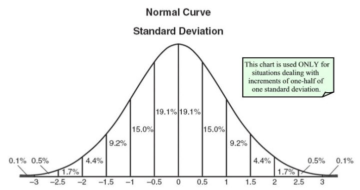
Chart prepared by the NY State Education Department

A chart, such as that seen above, is often used when dealing with normal distribution questions.  Understand that this chart shows only percentages that correspond to subdivisions up to one-half of one standard deviation.  Percentages for other subdivisions require a statistical mathematical table or a graphing calculator.  (See example 4)

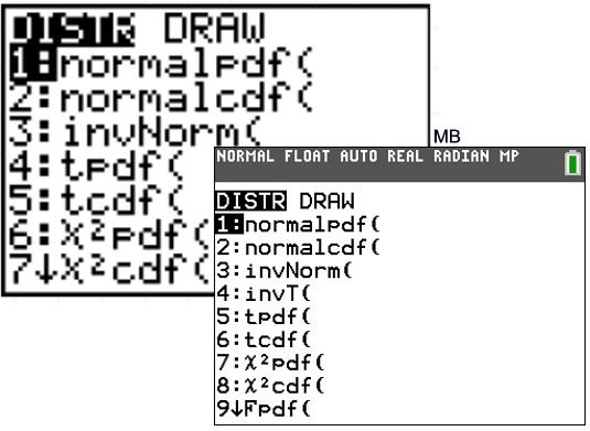
The Normal Probability Distribution menu for the TI-84+ is found under DISTR (2nd VARS). NOTE: A mean of zero and a standard deviation of one are considered to be the default values for a normal distribution on the calculator, if you choose not to set these values.

The Normal Distribution functions: #1: normalpdf pdf = Probability Density Function This function returns the probability of a single value of the random variable x.  Use this to graph a normal curve.Using this function returns the y-coordinates of the normal curve. Syntax:  normalpdf (x, mean, standard deviation) #2: normalcdf    cdf = Cumulative Distribution Function This function returns the cumulative probability from zero up to some input value of the random variable x.   Technically, it returns the percentage of area under a continuous distribution curve from negative infinity to the x.  You can, however, set the lower bound. Syntax: normalcdf (lower bound, upper bound, mean, standard deviation) #3: invNorm( inv = Inverse Normal Probability Distribution Function This function returns the x-value given the probability region to the left of the x-value. (0 < area < 1 must be true.)  The inverse normal probability distribution function will find the precise value at a given percent based upon the mean and standard deviation. Syntax:  invNorm (probability, mean, standard deviation)

Example 1:
Given a normal distribution of values for which the mean is 70 and the standard deviation is 4.5.  Find:
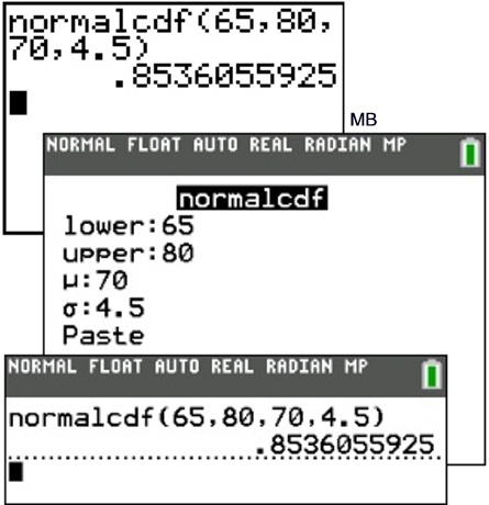
a) the probability that a value is between 65 and 80, inclusive.
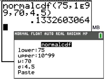
b) the probability that a value is greater than or equal to 75.
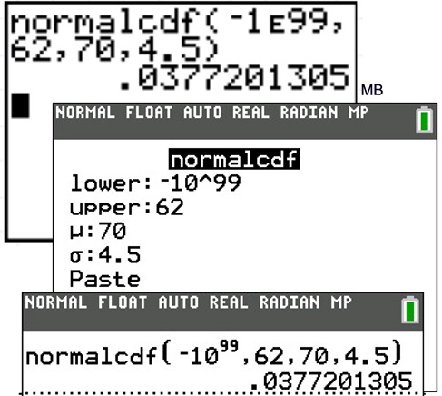
c) the probability that a value is less than 62.
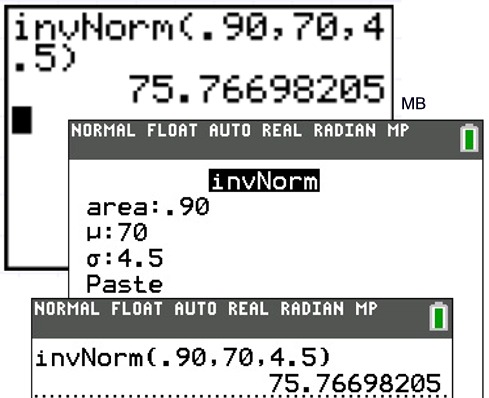
d) the 90^th percentile for this distribution.
       (answers will be rounded to the nearest thousandth)

1a:   Find the probability that a value is between 65 and 80, inclusive. (This is accomplished by finding the probability of the cumulative interval from 65 to 80.) Syntax: normalcdf(lower bound, upper bound, mean, standard deviation) Answer:   The probability is 85.361%. (The "PASTE" command simply means that the values that you typed after the template prompts will be "pasted" into the normalcdf() function and will appear on the home screen, as shown.)
1b: Find the probability that a value is greater than or equal to 75. (The upper boundary in this problem will be positive infinity.  The largest value the calculator can handle is 1 x 1099 .  Type 10^99 to represent postive infinity, [or type 1 EE 99.  Enter the EE by pressing 2nd, comma -- only one E will show on the screen.] Answer:  The probability is 13.326%.
1c:   Find the probability that a value is less than 62. (The lower boundary in this problem will be negative infinity.  The smallest value the calculator can handle is -1 x 1099 Type -10 ^ 99 [or type -1 EE 99.  Enter the EE by pressing 2nd, comma -- only one E will show on the screen.] Answer:  The probability is 3.772%.
1d: Find the 90th percentile for this distribution. (Given a probability region to the left of a value (i.e., a percentile), determine the value using invNorm.) Answer:  The x-value is 75.767.

Example 2:
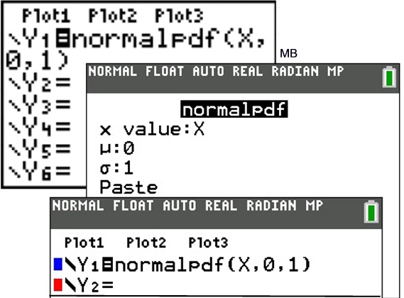
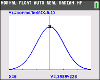
Graph and investigate the normal distribution curve where the mean is 0 and the standard deviation is 1.

For graphing the normal distribution, choose normalpdf. The normalpdf (normal probability density function) is found under DISTR (2nd VARS) #1normalpdf(.
Go to the Y = menu. The parameters will be (variable, mean, standard deviation).	Adjust the WINDOW. You will have to set your own window. Guideline is: Xmin = mean - 3 SD Xmax = mean + 3 SD Xscl = SD Ymin = 0 Ymax = 1/(2 SD) Yscl = 0	GRAPH.  Using TRACE, simply type the desired x value and the point will be plotted.
Investigate: What happens to the curve as the standard deviation increases?
Double the standard deviation and see what happens to the graph.	When graphing 2 normal curves, the window will need to be adjusted. Xmin = mean - 3 (largest SD) Xmax = mean + 3 (largest SD) Xscl = largest SD Ymin = 0 Ymax = 1/(2 smallest SD) Yscl = 0	Observe that as the standard deviation increases, the more spread out the graph becomes.
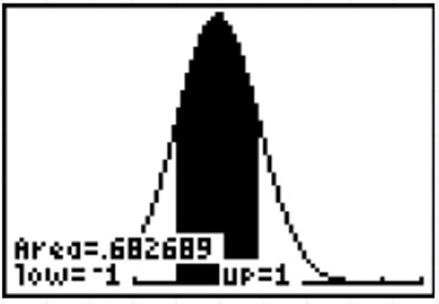
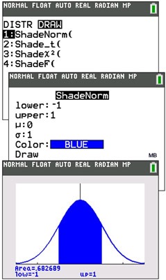
Now, the area under the curve between particular values represents the probabilities of events occurring within that specific range.  This area can be seen using the command ShadeNorm(. Before attempting ShadeNorm, be sure that Y1 = normalpdf(x, mean, standard deviation) is active and that the appropriate window has been set as indicated in the Window Guidelines in the previous section. To find ShadeNorm(, go to DISTR and right arrow to DRAW.   Choose #1:ShadeNorm(. ShadeNorm (lower bound, upperbound, mean, standard deviation) Notice that the calculator defaults to a mean of 0 and a standard deviation of 1 unless changed by the user. Remember that there is approximately a 68% probability of a score falling within 1 standard deviation from the mean in a normally distributed set of values. The "area" value in this graph is indicating 0.682689 or approximately 68%.
Notice how this answer supports the percentage listed in the chart at the top of this page.
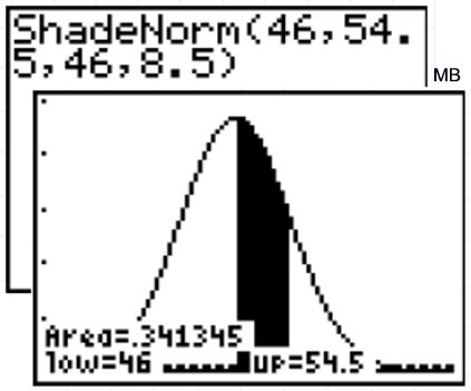
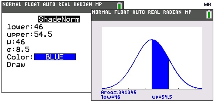
Example 3: Graph and examine a situation where the mean score is 46 and the standard deviation is 8.5 for a normally distributed set of data.
Go to Y= .	Adjust the window.	GRAPH.
Examine:  What is the probability of a value falling between the mean and the first standard deviation to the right? Answer:  approximately 34% Notice how this percentage supports the information found in the chart at the top of this page for the percentage of information falling within one standard deviation above the mean.

Example 4: The lifetime of a battery is normally distributed with a mean life of 40 hours and a standard deviation of 1.2 hours.  Find the probability that a randomly selected battery lasts longer than 42 hours.

pearceappeempa.blogspot.com

Source: https://mathbits.com/MathBits/TISection/Statistics2/normaldistribution.html

Share this post